General Help
 How do I register or subscribe?
To register, click on Subscribe, fill out the "New Users" information and press the "Register" button. Once registered, you can choose a subscription plan and immediately gain full access to all tools and features. Simply press the appropriate "Buy Now" button and proceed with check-out at the PayPal website. Note that you do not need a PayPal account, only a valid credit card. Your subscription will be active immediately after completion of the payment.
How do I register or subscribe?
To register, click on Subscribe, fill out the "New Users" information and press the "Register" button. Once registered, you can choose a subscription plan and immediately gain full access to all tools and features. Simply press the appropriate "Buy Now" button and proceed with check-out at the PayPal website. Note that you do not need a PayPal account, only a valid credit card. Your subscription will be active immediately after completion of the payment.
- What are the benefits of subscribing?
There are many benefits of becoming a subscriber. Some of the more popular features include the ability to simulate large wavebands, multiple gases and multiple gas cells. Subscribers have access to publication quality graphics and can download the raw data in text format. They can store their simulation setups for recall in later sessions. Subscribers can also upload their own custom line lists for testing and validation. Emission spectra can be computed with an optional blackbody source function, and instrument lineshape functions can be customized and applied to the spectra. Click here for a comparison of the features available with and without a subscription.
- What can I do for free?
The basic functionality of all the tools at SpectralCalc.com is freely available without subscribing. You can simulate transmittance spectra of gases with the same fast, accurate software used by many NASA remote sensing missions, and visually browse the HITRAN and other line list databases. The Blackbody Calculator, Atmosphere Browser and Solar Calculator are all freely available. Click here for a description of the many additional features available with a subscription.
- I can't use PayPal. How can I subscribe?
We can also accept checks and money orders. Please contact us, and we will arrange for a convenient payment solution.
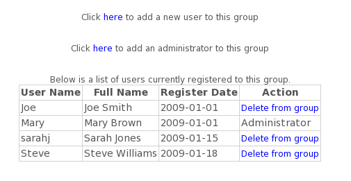
- How do I manage a group subscription?
Administrators can manage the group account from "My Account". Here you will see a list of all users currently in the group. You can add or delete users, and can designate an additional administrator if desired. Users can also join the group by logging in and entering the group code in "My Account".
Notes:
Users must be registered.
Group accounts can have up to 12 users, including the administrator(s).
Administrator(s) will receive email confirmation when a user joins the group.
A group account can have a maximum of 2 administrators.
Group codes are chosen by the administrator at time of purchase.
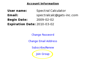
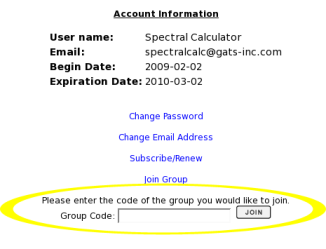
- How do I join a group?
To join a group account, go to "My Account" and click on "Join Group". Here you will be prompted to enter the group code. Contact the group administrator for this code.
Notes:Users must be registered.
Group accounts can have up to 12 users, including the administrator(s).
Administrator(s) will receive email confirmation when a user joins the group.
Group codes are chosen by the administrator at time of purchase.
- Details of SpectralCalc calculations
- Glossary
- Terms of Use
- Contact Us
- Testimonials
Simulation Tools
- Gas-Cell Simulator
- Gas-cell Simulator User Guide
- What does the Gas-cell Simulator do?
The Gas-cell Simulator models gas spectra. With just a few clicks you can accurately simulate the spectra of most of the important trace gas species in the Earth's atmosphere, such as water vapor, carbon dioxide, ozone, methane and dozens more. Spectra are calculated in the user-specified waveband with full resolution, fine enough to accurately capture the shape of even the narrowest molecular absorption line. The underlying software is scientifically rigorous and has been used in support of a number of NASA research projects.
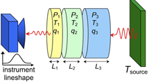
The basic setup models the transmittance through a "gas cell" -- an imaginary sealed container with transparent walls. The transmittance is simply the fraction of radiation that makes it through the gas cell. This is illustrated below.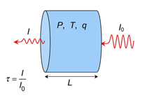
The transmittance, τ, is the ratio of the intensity of the transmitted radiation, I, to the incident, I0. You control the pressure, P, temperature, T and length, L, of the gas cell, the concentration of the absorbing gas inside, q, and the range of wavenumbers over which to compute the spectrum. The Gas-cell Simulator then accurately calculates the full-resolution transmittance spectrum.
Subscribers have access to some advanced features. They can simulate mixtures of several gases and can "stack" up to six gas cells end-to-end, controlling the conditions of each. They can choose to compute emission spectra rather than transmittance spectra, and add an optional blackbody source behind the gas cells. Instrument lineshape functions that "apodize" or smooth the spectra can also be included. These features are illustrated below.
Click here for a comprehensive list of features available to subscribers.
- How do I operate the Gas-cell Simulator?
Choose your waveband, set up your gas cells, and press Calculate! Many variations are possible, so we've divided the inputs into functional "tabs" to make things more manageable.
- Observer Tab - choose the waveband and any other instrument parameters
- Gas Cells Tab - specify the gases to simulate and gas cell conditions
- Source Tab (optional) - include a blackbody background
- Plot Options Tab (optional) - control plot features like log or linear scaling
- My Settings Tab (optional) - save and retrieve simulation setups
- How big of a waveband can I simulate?
Spectra with up to 1 million points can be calculated. The size of the waveband that this supports depends on the spectral resolution of the spectrum. In general, low pressure spectra have very narrow spectral features, and require very fine resolution, especially at low wavenumbers. (Note: the spectral resolution of an atmospheric path will be governed by its highest altitude.) Here are some typical examples:
scenario spectral range points atmospheric path, ground to space 1,000 – 1,100 cm-1 582,630 atmospheric path, ground to 1 km 1,000 – 1,100 cm-1 82,878 gas cell at 1,000 mbar 3,000 – 5,000 cm-1 611,820 gas cell at 0.001 mbar 3,000 – 3,500 cm-1 477,876 gas cell at 0.001 mbar 300 – 350 cm-1 477,834
- How is the spectral resolution determined?
The spectral resolution (point spacing in cm-1) is chosen to be fine enough to fully capture the line shape of the thinnest absorption line in the spectrum. Our software surveys all absorption lines needed and finds the smallest width. The spectral resolution is set to 20% of the thinnest line's halfwidth. In general, at pressures above 1 mbar, the lines are pressure broadened with widths proportional to pressure. At low pressures (below 1 mbar), only Doppler broadening is important, and the widths are proportional to wavenumber (position of line). A more detailed description is available here.
- I just need coarse spectra. How do I get this?
You can select an instrument function (Observer Tab) to model spectra as would be obtained from an instrument with a specified spectral resolution. Adjusting the width of the instrument function will control the resolution of the resulting spectrum. Please see the Instrument Function FAQ for details.
- What is an "Instrument Function"?
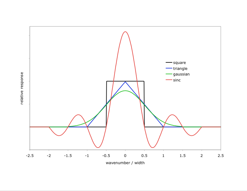
SpectralCalc models spectra at very fine resolution – fine enough to capture every significant spectral feature. We sometimes call these “monochromatic” spectra. Real instruments, however, always have some inherent resolution and produce somewhat smoothed spectra, effectively convolving the received monochromatic spectra with the instrument’s spectral response function. To simulate a spectrum with an instrument function, select the desired function type and width from the Observer Tab. The available types are shown here.
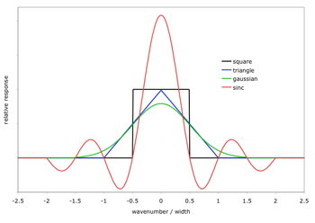
Click on the image to see a larger version
There are several important things to note when applying instrument functions:- The specified width must be less than 250 cm-1 and less than 1/10th of the waveband. The width can be arbitrarily small, but widths smaller than the inherent resolution of the underlying spectrum are ignored.
- Larger widths produce coarser spectra (40 points per instrument function width), but the underlying calculation is always done at high spectral resolution.
- Instrument functions are computed and applied in wavenumbers. A width specified in microns is converted to the equivalent width in wavenumbers at the center of the bandpass. As a result, an instrument function with its width specified in microns will actually have different effective widths in different spectral bandpasses.
- Instrument functions should only be applied to the final spectrum. For example, to model the combined spectrum of sequential absorbing paths, we should compute and save the monochromatic transmittance spectra of each. Then on the My Spectra Tab, we can compute their product, and finally apply an instrument function to the resulting monochromatic spectrum. Applying the instrument function to the individual spectra and then combining them will produce erroneous results.
- Instrument Functions Information
- How does the Gas-cell Simulator model the spectra?
The Gas-cell Simulator uses a line-by-line model called LinePakTM to accurately model the spectra of molecular absorption lines. The shape, position and depth of each line are described by parameters in a line list such as HITRAN, and adjusted for the user-specified pressure, temperature, and gas concentration. We maintain an up-to-date copy of the HITRAN line parameters, and allow alternate line lists to be used as well. Details of the calculation are given here.
- Why do I only have to specify the length of the gas cell, not its volume?
The length of the gas cell is the only dimension that matters because the simulation is of a single beam through the gas cell. Only molecules along the line-of-sight will affect this radiation.
- What line shape is used in the computation?
At all but very low wavenumbers, the LinePakTM software uses the Voigt profile. The Voigt profile combines the pressure-induced line broadening effects of molecular collisions, and the thermal-induced Doppler effect resulting from their randomly oriented motions. At very low wavenumbers (below 200 cm-1) the Van Vleck Weisskopf line shape is used.
LinePakTM can easily accommodate more complex line shapes, such as the Galatry or speed-dependent profiles, but the spectroscopic parameters needed for these are currently available only for a small number of absorption lines. Note that these provide only a very small improvement, and in most situations, the Voigt profile adds no significant error.
- Do you include effects from absorption lines outside my spectral bandpass?
Yes. In many situations, the spectrum in a specified bandpass will have significant contributions from absorption lines centered outside the bandpass. To ensure that this is modeled correctly, the Gas-cell Simulator software calculates the spectra over a larger waveband, extended by 120 cm-1 on either side of the specified range.
- How can I compare the Gas-cell Simulator results to a spectrum measured in air?
The Gas-cell Simulator reports spectra as would be measured in vacuum. (Outside the gas cell a vacuum is assumed). In some applications, spectra are measured in air. Because the speed of light is slower in air than in vacuum, the observed wavenumber (1/c in cm-1) is slightly larger than it would have been if it had been observed in vacuum. To compare Gas-cell Simulator results to spectra measured in air (or some other media), this shift must be accounted for.
- What is the relative abundance of a particular isotopologue?
The Gas-cell Simulator assumes the same natural abundances of the various isotopologues as HITRAN. Click here to view the list of assumed abundances.
- Can I simulate different isotopologues?
Yes. On the Gas Cell calculator, select the isotopologue to be simulated and specify the desired abundance. You can simulate mixtures of different isotopologues and control the concentration of each. Note: If “All” isotopologues are selected for a molecule, they are automatically scaled by their natural abundance so that they sum to the specified VMR.
- How can I simulate isotopic mixtures?
Each isotopologue has a unique spectrum and must be simulated separately. Unless the user specifies otherwise, it is assumed that the gas sample includes all isotopologues of the specified molecule, in their natural abundances. The natural abundances are implicitly accounted for in our calculations by pre-scaling the spectral line intensities.
To simulate spectra of a single isotopologue, or a sample with an elevated concentration of a minor isotopologue, simply switch the isotopologue drop-down menu from All to the desired isotopologue. When a specific isotopologue is simulated, our software removes the pre-scaling from the HITRAN line intensities, so that the simulation reflects the concentration supplied by the user.
- Are effects other than molecular line absorption/emission included?
Yes, continuum absorption/emission for N2, O2 and H2O are included. These effects are automatically included as needed for simulations involving these molecules. Other effects, such as Rayleigh (molecular) and Mie (particulate) scattering, are not yet included.
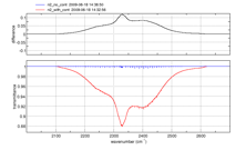
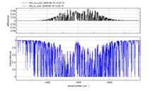
- How are continua modeled?
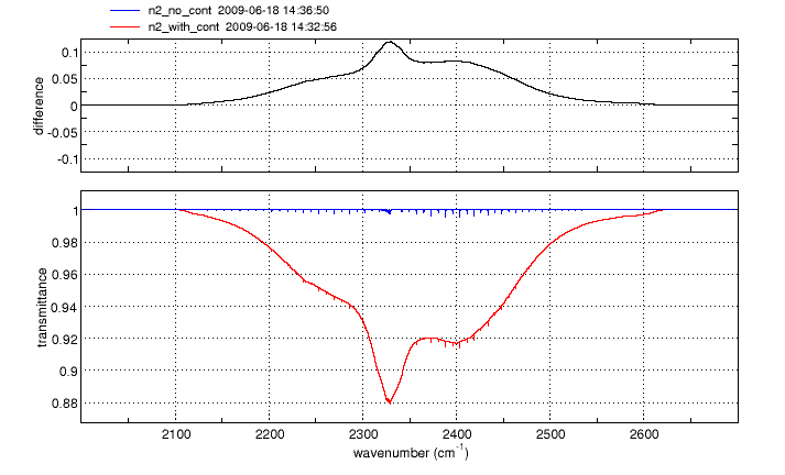
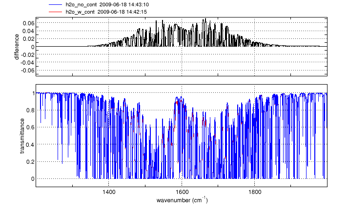
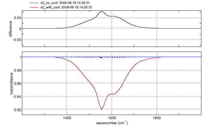
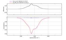
Continuum absorption/emission effects for N2, O2 and H2O are modeled using the approaches described by Clough, et al. [1] and Lafferty et al. [2]. These continuum models augment the standard "line-by-line" calculation, more accurately accounting for far-wing effects at high pressures.
For O2 and N2, the spectral ranges affected are 1345-1820 cm-1 and 2105-2620 cm-1 respectively. The H2O continuum is significant at wavenumbers below 600 cm-1 and between 1200 and 2000 cm-1.
Click on an image to see a larger version
Gas cell simulations of N2, O2 and H2O spectra in any of the above wavebands will automatically include the appropriate continuum model(s). No action is needed from the user.
For all three gases, the effect is proportional to pressure, and is negligible at pressures less than ~10mbar. Temperature dependence of the continua is included in the model, derived from laboratory measurements between 70 and 350 K. Continuum absorption for spectra at higher temperatures is based on extrapolation of these data, and therefore may contain some inaccuracies. Note, however that the continuum effects are inversely proportional to temperature, so the overall magnitude become negligible for high temperatures.
[1] Clough, S. A., F. X. Kneizys, and R. W. Davies, "Lineshape and the water vapor continuum," Atmos. Res. 23, 229-241 (1989)
[2] Lafferty, W. J., A. M. Solodov, A. Weber, W. B. Olson, and J. Hartmann, "Infrared collision-induced absorption by N2 near 4.3 µm for atmospheric applications: measurements and empirical modeling," Appl. Opt. 35, 5911-5917 (1996)
- The Gas-cell Simulator says "No absorption lines found." What did I do wrong?
Maybe nothing. This simply means there are no absorption lines for the selected gas in the specified waveband. You may wish to visit the Line List Browser to identify spectral regions in which each gas does have absorption lines, and adjust your waveband and/or gas accordingly.
- An error message says my spectrum has too many points. What should I do?
The total number of points in a spectrum is the waveband size divided by the spectral resolution (point spacing in cm-1). There are several things you can do to reduce the total number of points:
- Reduce the waveband. This will directly reduce the number of points. In general, the lower wavenumber regions require the most points.
- Increase the pressure. Gases at low pressure (< 0.1 mbar) have very thin Doppler-broadened lines, and require very fine spacing in the calculation.
- Limit the altitude of atmospheric paths. High altitudes have low pressures, and thus need fine resolution. Restricting your path to low altitudes should help.
- Avoid low wavenumbers at low pressure. At low-pressure, absorption lines have Doppler widths proportional to wavenumber, so low wavenumber/low pressure spectral calculations are particularly difficult.
In some situations, the calculation may need to be split up into a number of spectral segments, and each calculated individually.
- Can I prove or disprove global warming with SpectralCalc.com?
Of course not. However, SpectralCalc can be used to demonstrate some of the fundamental principles. Spectroscopy of greenhouse gases is critical in atmospheric modeling, and SpectralCalc accurately simulates high-resolution molecular spectra of atmospheric paths (currently for Earth or Mars). Still, while these simulations are useful and important, any sufficiently complete climate model has to include a host of other significant components, including surface albedo, clouds and aerosols, solar variability and ocean cycles. For more details on atmospheric climate modeling, a nice introduction is available here: http://geosci.uchicago.edu/~rtp1/papers/PhysTodayRT2011.pdf
- Is there a publication describing the calculation?
Yes. The underlying algorithm was first described in the following paper: Gordley et al., LINEPAK: Algorithm for Modeling Spectral Transmittance and Radiance, J. Quant. Spectrosc. Radiat. Transfer Vol. 52, No. 5, pp.563-580, 1994
- Atmospheric Paths
- Atmospheric Paths User Guide
- How is the atmosphere modeled?
The atmosphere is modeled as graduated concentric spherical shells. The number of shells depends on the path length and altitude range. For example, a path from the ground to 120 km (the top of our model atmospheres) is split into 19 shells: 250 meters thick at the surface, growing to 10 km thick at high altitudes. The temperature and gas concentrations in each shell are taken from the selected model atmosphere. These model data can be viewed/downloaded with the Atmosphere Browser tool. Within each shell, a mass-weighted computation is performed, as described by Gordley and Marshall. Refraction effects are rigorously included in all paths. (Note that radiance spectra for up-looking and downlooking paths are different, whereas transmittance spectra are the same for both directions.)
- What line shape is used in the computation?
At all but very low wavenumbers, the LinePakTM software uses the Voigt profile. The Voigt profile combines the pressure-induced line broadening effects of molecular collisions, and the thermal-induced Doppler effect resulting from their randomly oriented motions. At very low wavenumbers (below 200 cm-1) the Van Vleck Weisskopf line shape is used.
LinePakTM can easily accommodate more complex line shapes, such as the Galatry or speed-dependent profiles, but the spectroscopic parameters needed for these are currently available only for a small number of absorption lines. Note that these provide only a very small improvement, and in most situations, the Voigt profile adds no significant error.
- How is the spectral resolution determined?
The spectral resolution (point spacing in cm-1) is chosen to be fine enough to fully capture the line shape of the thinnest absorption line in the spectrum. Our software surveys all absorption lines needed and finds the smallest width. The spectral resolution is set to 20% of the thinnest line's halfwidth. In general, at pressures above 1 mbar, the lines are pressure broadened with widths proportional to pressure. At low pressures (below 1 mbar), only Doppler broadening is important, and the widths are proportional to wavenumber (position of line). A more detailed description is available here.
- I just need coarse spectra. How do I get this?
You can select an instrument function (Observer Tab) to model spectra as would be obtained from an instrument with a specified spectral resolution. Adjusting the width of the instrument function will control the resolution of the resulting spectrum. Please see the Instrument Function FAQ for details.
- Do you include effects from absorption lines outside my spectral bandpass?
Yes. In many situations, the spectrum in a specified bandpass will have significant contributions from absorption lines centered outside the bandpass. To ensure that this is modeled correctly, the Gas-cell Simulator software calculates the spectra over a larger waveband, extended by 120 cm-1 on either side of the specified range.
- How big of a waveband can I simulate?
Spectra with up to 1 million points can be calculated. The size of the waveband that this supports depends on the spectral resolution of the spectrum. In general, low pressure spectra have very narrow spectral features, and require very fine resolution, especially at low wavenumbers. (Note: the spectral resolution of an atmospheric path will be governed by its highest altitude.) Here are some typical examples:
scenario spectral range points atmospheric path, ground to space 1,000 – 1,100 cm-1 582,630 atmospheric path, ground to 1 km 1,000 – 1,100 cm-1 82,878 gas cell at 1,000 mbar 3,000 – 5,000 cm-1 611,820 gas cell at 0.001 mbar 3,000 – 3,500 cm-1 477,876 gas cell at 0.001 mbar 300 – 350 cm-1 477,834
- Can I simulate different isotopologues?
Atmospheric path calculations automatically account for the natural abundance of each isotopologue. You can add an individual isotopologue as one of your six species to further control its concentration. Note: all isotopologues of a molecule have the same vertical structure, with their individual concentrations scaled everywhere by their natural abundance. The vertical profiles of all species are available in the Atmosphere Browser.
- What is an "Instrument Function"?
SpectralCalc models spectra at very fine resolution – fine enough to capture every significant spectral feature. We sometimes call these “monochromatic” spectra. Real instruments, however, always have some inherent resolution and produce somewhat smoothed spectra, effectively convolving the received monochromatic spectra with the instrument’s spectral response function. To simulate a spectrum with an instrument function, select the desired function type and width from the Observer Tab. The available types are shown here.
Click on the image to see a larger version
There are several important things to note when applying instrument functions:- The specified width must be less than 250 cm-1 and less than 1/10th of the waveband. The width can be arbitrarily small, but widths smaller than the inherent resolution of the underlying spectrum are ignored.
- Larger widths produce coarser spectra (40 points per instrument function width), but the underlying calculation is always done at high spectral resolution.
- Instrument functions are computed and applied in wavenumbers. A width specified in microns is converted to the equivalent width in wavenumbers at the center of the bandpass. As a result, an instrument function with its width specified in microns will actually have different effective widths in different spectral bandpasses.
- Instrument functions should only be applied to the final spectrum. For example, to model the combined spectrum of sequential absorbing paths, we should compute and save the monochromatic transmittance spectra of each. Then on the My Spectra Tab, we can compute their product, and finally apply an instrument function to the resulting monochromatic spectrum. Applying the instrument function to the individual spectra and then combining them will produce erroneous results.
- Instrument Functions Information
- Are effects other than molecular line absorption/emission included?
Yes, continuum absorption/emission for N2, O2 and H2O are included. These effects are automatically included as needed for simulations involving these molecules. Other effects, such as Rayleigh (molecular) and Mie (particulate) scattering, are not yet included.
- How are continua modeled?
Continuum absorption/emission effects for N2, O2 and H2O are modeled using the approaches described by Clough, et al. [1] and Lafferty et al. [2]. These continuum models augment the standard "line-by-line" calculation, more accurately accounting for far-wing effects at high pressures.
For O2 and N2, the spectral ranges affected are 1345-1820 cm-1 and 2105-2620 cm-1 respectively. The H2O continuum is significant at wavenumbers below 600 cm-1 and between 1200 and 2000 cm-1.
Click on an image to see a larger version
Gas cell simulations of N2, O2 and H2O spectra in any of the above wavebands will automatically include the appropriate continuum model(s). No action is needed from the user.
For all three gases, the effect is proportional to pressure, and is negligible at pressures less than ~10mbar. Temperature dependence of the continua is included in the model, derived from laboratory measurements between 70 and 350 K. Continuum absorption for spectra at higher temperatures is based on extrapolation of these data, and therefore may contain some inaccuracies. Note, however that the continuum effects are inversely proportional to temperature, so the overall magnitude become negligible for high temperatures.
[1] Clough, S. A., F. X. Kneizys, and R. W. Davies, "Lineshape and the water vapor continuum," Atmos. Res. 23, 229-241 (1989)
[2] Lafferty, W. J., A. M. Solodov, A. Weber, W. B. Olson, and J. Hartmann, "Infrared collision-induced absorption by N2 near 4.3 µm for atmospheric applications: measurements and empirical modeling," Appl. Opt. 35, 5911-5917 (1996)
- How high do the atmosphere models go?
The atmosphere models extend to 120 km. If the observer height or target height is above this altitude, the portion of the atmosphere above 120 km is represented by an isothermal layer with the same temperature and VMR conditions as 120 km. The pressure in this layer is hydrostatically decreasing and extends for 3 scale heights.
- What is the tangent height?
The tangent height of a limb path is the altitude of its closest approach to the Earth’s surface. Atmospheric refraction bends the path, and the refracted tangent height is lower than the “apparent” tangent height, as shown here:
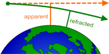
The user supplies the apparent tangent height. SpectralCalc calculates the refracted tangent height. Refraction is more severe at low altitudes, and depends somewhat on the model atmosphere. Rays with very low apparent tangent heights may intersect the Earth. In this case, an error message is displayed, and you will need to increase the apparent tangent height until the refracted ray does not hit the Earth.
- How can I simulate isotopic mixtures?
Each isotopologue has a unique spectrum and must be simulated separately. Unless the user specifies otherwise, it is assumed that the gas sample includes all isotopologues of the specified molecule, in their natural abundances. The natural abundances are implicitly accounted for in our calculations by pre-scaling the spectral line intensities.
To simulate spectra of a single isotopologue, or a sample with an elevated concentration of a minor isotopologue, simply switch the isotopologue drop-down menu from All to the desired isotopologue. When a specific isotopologue is simulated, our software removes the pre-scaling from the HITRAN line intensities, so that the simulation reflects the concentration supplied by the user. - The Atmospheric Paths Tool says "No absorption lines found." What did I do wrong?
Maybe nothing. This simply means there are no absorption lines for the selected gas in the specified waveband. You may wish to visit the Line List Browser to identify spectral regions in which each gas does have absorption lines, and adjust your waveband and/or gas accordingly.
- An error message says my spectrum has too many points. What should I do?
The total number of points in a spectrum is the waveband size divided by the spectral resolution (point spacing in cm-1). There are several things you can do to reduce the total number of points:
- Reduce the waveband. This will directly reduce the number of points. In general, the lower wavenumber regions require the most points.
- Increase the pressure. Gases at low pressure (< 0.1 mbar) have very thin Doppler-broadened lines, and require very fine spacing in the calculation.
- Limit the altitude of atmospheric paths. High altitudes have low pressures, and thus need fine resolution. Restricting your path to low altitudes should help.
- Avoid low wavenumbers at low pressure. At low-pressure, absorption lines have Doppler widths proportional to wavenumber, so low wavenumber/low pressure spectral calculations are particularly difficult.
In some situations, the calculation may need to be split up into a number of spectral segments, and each calculated individually.
- Can I prove or disprove global warming with SpectralCalc.com?
Of course not. However, SpectralCalc can be used to demonstrate some of the fundamental principles. Spectroscopy of greenhouse gases is critical in atmospheric modeling, and SpectralCalc accurately simulates high-resolution molecular spectra of atmospheric paths (currently for Earth or Mars). Still, while these simulations are useful and important, any sufficiently complete climate model has to include a host of other significant components, including surface albedo, clouds and aerosols, solar variability and ocean cycles. For more details on atmospheric climate modeling, a nice introduction is available here: http://geosci.uchicago.edu/~rtp1/papers/PhysTodayRT2011.pdf
- Is there a publication describing the calculation?
Yes. The underlying algorithm was first described in the following paper: Gordley et al., LINEPAK: Algorithm for Modeling Spectral Transmittance and Radiance, J. Quant. Spectrosc. Radiat. Transfer Vol. 52, No. 5, pp.563-580, 1994
- My Spectra
- How can I import my own spectra?
Subscribers can import their transmittance or radiance spectra by using the Upload tab on the My Spectra tool. Enter the full name (including directory path) of the file to upload, or use the Browse button to locate the file on your computer. Choose a short descriptive name to identify the spectrum, and select Transmittance or Radiance for the spectrum type. A description of the file can be typed into the text box provided. Once uploaded, the spectrum will be available on the My Spectra tab, where it can be viewed, downloaded, deleted, etc. (Other users do not have access to your stored spectra.)
File requirements: The uploaded spectrum file must be in plain text format with two columns, the first column containing the wavenumber (cm-1) values, and the second containing the transmittance or radiance values (W/m2/sr/cm-1). Files must be no bigger than 20 MB, and contain no more than 400,000 spectral points. Header lines (lines that begin with something other than a space, a digit or a decimal point) are allowed at the beginning of the file, but are ignored. The columns can be space-, tab- or comma-delimited. Any text following the second column is ignored. Wavenumbers are assumed to be equally spaced and increasing. Wavenumber spacing must be in the range 1e-8 to 100 cm-1. (Only the first and last wavenumber are actually stored. The grid is reconstructed each time the data are retrieved from our database.) Transmittance values must be between -1 and 2, and radiance values must be between 0 and 1000 W/m2/sr/cm-1.
- Line List Browser
- What does the Line List Browser do?
The Line List browser lets you quickly and easily see where gases have absorption lines, and how strongly they absorb, without the time and effort of performing a detailed simulation. This tool displays the contents of HITRAN, GEISA and other line list databases. You can also download the line list data here, selecting the complete datasets or just the molecules and wavebands you want.
- How can I import my own line list?
Subscribers can import their own spectral line lists using the My Line Lists tab on the Linelist Browser tool. The line list must be a text file in HITRAN format. Up to 100,000 lines are allowed. The list can include only molecules/isotopologues that are already in the public HITRAN distribution. (If you have line parameters for molecules/isotopologues not in HITRAN, please contact us and we will help get your data uploaded.) It can take several minutes for the conversion, validation and upload process. Once your data is uploaded, your line list will be visible under My Line Lists and available for browsing or spectral calculations. Other subscribers will not be able to access your line lists.
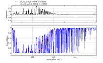
- What is "line intensity"?
Line intensity is a parameter that indicates the strength of a spectral line. These are used in our simulations to compute absorption and emission spectra. The Line List Browser shows the line intensities of each molecule in a spectral range. Viewing the line intensities gives a quick indication of the spectrum of the chosen molecule(s), without having to perform any lengthy calculations. This is very useful for determining which molecules absorb in a particular waveband, or for identifying spectral lines in measured spectra. A detailed description of how these intensities are used in the simulation of a spectrum is available here.
Because molecular species have widely differing concentrations in the atmosphere, we offer the option of plotting intensities scaled by the atmospheric concentration (in molecules per cm3). Simply choose an atmosphere model and altitude, and the line intensities will be scaled by the species’ concentrations at that altitude. The raw intensities, as supplied by HITRAN and other databases, have units of cm-1/(molecule/cm-2) at 296 K, while the scaled line intensities have units of cm-1/cm (wavenumber per unit path length).
When plotting line intensities of individual isotopologues of a molecule, you have the option of plotting the intensities with or without scaling by their natural abundance.
- What are cross section spectra used for?
Cross sections are normalized molecular absorption spectra. These are often used to simulate broad absorption features that are not well modeled using line-by-line techniques, or for which adequate line parameters are not available. Cross section spectra are typically given in units of cm2 per molecule at each wavenumber.
Infrared spectra of polyatomic "heavy" molecules such as CFCs, and UV absorption features of several important atmospheric species, most notably ozone, are better simulated using cross sections than line-by-line models. Cross section spectra for these molecules can be accessed in the Line List Browser, by selecting Plot Type-->Cross Sections.
We're working on integrating the capability of simulating spectra using cross sections to our online tools, but have not yet validated and tested a general-purpose interface for this.
- Why are Line Intensities Pre-scaled in HITRAN?
To make the simulation of atmospheric spectra more efficient, HITRAN and other databases have pre-scaled the spectral line intensities for each isotopologue by the natural abundance of the isotopologue. For example, the line intensities for the primary carbon dioxide isotopologue (16O12C16O) are scaled by a factor of 0.984204, whereas the line intensities of the secondary isotopologue (16O13C16O) are scaled by a much smaller factor, 0.0110574. This pre-scaling implicitly accounts for the relative concentration of the various isotopologues in atmospheric gases, making line-by-line calculations more efficient. In the event a single isotopologue is to be simulated, our software simply “unscales” the line-intensities from HITRAN (or other database) before proceeding with the calculation of the spectrum.
Note: any linelists uploaded by users are assumed to be pre-scaled in this same manner. - Blackbody Calculator
- Atmosphere Browser
- Atmosphere Browser User Guide
- How high do the atmosphere models go?
The atmosphere models extend to 120 km. If the observer height or target height is above this altitude, the portion of the atmosphere above 120 km is represented by an isothermal layer with the same temperature and VMR conditions as 120 km. The pressure in this layer is hydrostatically decreasing and extends for 3 scale heights.
- Solar Calculator