User Guide for the Atmospheric Paths Tool on SpectralCalc.com
Note: The Atmospheric Paths tool is computationally intensive, and available only to active subscribers. It’s quick and easy to subscribe Non-subscribers can model simpler scenarios using the Gas Cell tool.
Getting Started
Log in at www.spectralcalc.com, choose your waveband, pick a path geometry, and press Calculate! It’s that simple. We’ve pre-filled all inputs with reasonable default values, so it works “right out of the box.” Of course, you will likely want to do something different than the default scenario, and there are many possible variations. To make it easy, we've grouped the controls into functional “Tabs”:
Observer set the waveband, calculation type and instrument resolution
Atmosphere specify the path geometry, atmosphere model and line list
Source adjust the background temperature and emissivity
Plot Options control plot features like log or linear scaling
My Settings save and retrieve your stored simulation setups
Each of these is fully described in the Configuring Inputs section below, but typically only a few parameters will need to be adjusted from their default values.
Calculate
Once you have configured any inputs that need adjustment, press the Calculate button. A plot of your spectrum will appear. Most calculations take only a few seconds, but some more intensive computations can take up to a minute or more. (You may need to scroll down in your browser window to view the spectrum.) Subsequent calculations will "push down" any earlier plots. If any inputs are out of the acceptable ranges, a red text message will appear, and an X will be placed next to the offending input value(s). Note: the offending input may be on a Tab that is not visible, so you may have to look through several Tabs to locate the problem.
Clear Plots
This erases all plots from the page. Note: once the plots are cleared, access to the postscript, PDF and text files cannot be recovered. Before clearing the plots, make sure you have saved any plots or data that you may want to keep. Methods for saving data are described in the Post Calculation Options section, below.
Reset All
Press this button to erase all plots from the page and reset inputs on all tabs to their default values. Once pressed, Postscript, PDF, text files and all input data will no longer be available, so make sure you have saved any plots or data that you may want to keep. Methods for saving data are described in the Post Calculation Options section, below.
Configuring Inputs
As mentioned above, we've grouped the controls into functional "Tabs" and pre-filled every input with a reasonable value. This makes setting up your calculation quick and efficient. In most cases, you will only need to visit the Observer and Atmosphere Tabs and adjust a few values.
Observer Tab
The inputs here describe the hypothetical "instrument" that will measure your spectrum. You can think the instrument as ideal spectrometer, with infinitely fine resolution or with a specified instrumental lineshape, if desired.
Transmittance or Emission/radiance - You can choose to calculate either the transmittance or emission spectrum. By default, the transmittance spectrum is computed. Transmittance is the ratio of transmitted light intensity to incident light intensity. Emission is the spectral radiance received (e.g. W/m2/sr/cm-1 or W/m2/sr/micron) from the molecules in the path and a blackbody at the far end. If emission is selected, by default a blackbody target will be inserted at the same temperature as its surrounding atmosphere. The target temperature and emissivity can be adjusted from the Source Tab
Waveband - Specify the units (cm-1 or microns), and limits of the waveband to be observed. Both lower and upper limits must be between 0 and 60,000 cm-1. The waveband size (upper limit - lower limit) must be small enough to ensure the computations will be completed in a reasonable amount of time, and the resulting files will be of manageable size. The maximum waveband size depends on the scenario being modeled. More details can be found here.
Note that the resulting spectrum may have endpoints that are slightly offset from the specified limits. This is simply the result of our adaptive algorithm for determining the spectral resolution. Note also that features centered outside the waveband often influence the spectrum in the waveband. To capture such effects, our algorithm includes any transition within 100 cm-1 of the specified waveband.
Instrument Function - Select an apodizing instrument function (i.e. an instrumental lineshape) and specify its width. The calculated high-resolution spectrum will be convolved with the selected instrument function. Instrument lineshape functions are described here. The larger the width, the coarser the resulting spectrum and smaller the file size will be. A word of caution: Generally, the unapodized, high-resolution spectra are needed for post processing applications. For example, modeling the effect of a spectral filter in a system entails the point-by-point multiplication of the high-resolution spectrum with the filter response, and convolving this product with the instrument function. Apodizing the spectrum prior to the multiplication is incorrect, and may introduce significant error.
Atmosphere Tab
Scenarios – There are several scenarios, or path types, available for simulation:
Horizontal: In this scenario, the atmosphere is modeled as a single gas cell. No Earth curvature is included. Conditions of the cell are determined by the chosen atmosphere model and specified height.
Up Looking: This describes a path from the observer to a target (source) at some higher altitude. The Zenith Angle is the angle between straight up and the target’s apparent (unrefracted) direction. The target height must be at least 1 km higher than the observer. When simulating emission, targets in the atmosphere (height <120 km) are treated by default as blackbodies at the atmospheric temperature. For targets above the atmosphere, no target radiance is included by default. The target temperature can be adjusted in the Source Tab.
Down Looking: This models a path from the observer to a target (source) at some lower altitude. The Nadir Angle is the angle between straight down and the target’s apparent (unrefracted) direction. The target height must be at least 1 km lower than the observer. Nadir angles must be small enough so that the direction intersects the Earth. When simulating radiance, the target is by default modeled as a blackbody at the atmospheric temperature. You can adjust the target temperature in the Source Tab.
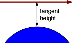
Limb Path: This models a path through the entire limb of the atmosphere. The tangent height is the minimum height of the apparent (unrefracted) path. Refraction will be rigorously modeled in the calculation and the true (refracted) tangent height will be noted in the text file. Both observer and target are assumed exoatmospheric. When simulating radiance, by default no target radiance is included, but this can be adjusted in the Source Tab. An error message will be reported if the refracted path intersects the Earth. In this case, you will need to increase the tangent height value.
Line List – This drop-down menu controls which set of spectral line parameters will be used to model the molecular absorption/emission lines. For example, you may select HITRAN, GEISA, HITEMP or any custom line list that you have previously uploaded. Custom line lists can be imported from the Line List Browser tool.
Model Atmosphere – Select a model atmosphere from this drop-down menu. Each model atmosphere contains temperature, pressure and gas concentrations at all altitudes. Use the Atmosphere Browser tool to create new atmospheres, plot profiles or download the raw data.
Gases / Isotopologues – The most common species are selected by default, but you can choose any six gases from our database. If “All” is selected from the isotopologue menu, a mixture of all cataloged isotopologues for that species will be simulated, each with it’s natural abundance (see here for tables of abundances). To simulate an individual isotopologue, select the desired formula from the isotopologue drop-down menu. For example, choosing two species, “H2O - All” and “H2O 4 HD(16)O” will simulate an atmosphere with enhanced HDO.
Scale Factor – Here you can adjust the concentrations of each gas. The entire vertical profile of the gas (i.e. its concentration at every altitude) will be multiplied by the specified scale factor. For example, specifying a scale factor of 1.5 for a gas will increase its concentration by 50% at every altitude. A scale factor of 0 effectively removes that gas from the path. You can view the nominal vertical profiles of each species in each model atmosphere with the Atmosphere Browser tool. All scale factors must be between 0 and 1000. An error message will be reported if the scaled mixing ratio value for any included gas exceeds 1 or the sum of their vmrs exceeds one. In this case, you will need to reduce the value of the scaling factor.
Source Tab
Radiance (emission) spectra can include the contribution from a background source or target (such as the Earth’s surface), but by default the source radiance is turned off. To have source radiance included in the simulation, simply switch the Blackbody Source “On” in the Source tab. You can then select its temperature and emissivity. When enabled, the simulated spectrum will include the radiance of a blackbody located at the end of the specified path, attenuated by the intervening atmosphere. For example, to include the radiance of the Earth in a downlooking scenario, you must turn the Blackbody Source “On” and adjust the temperature to the desired value. (Note: temperature must be between 0.1 and 20,000 K, and emissivity between 0 and 1.)
Plot Options Tab
Various aspects of the plot appearance can be controlled here.
Plot Line intensities - Checking this box will add a secondary graph above the main spectrum graph. This secondary graph shows the individual absorption lines as "sticks" with height equal to the line strength. Multiple species are plotted in different colors. This can help reveal which species is responsible for a particular feature in the spectrum.
Log Scale - Checking this box sets the scale of the vertical (radiance) axis on emission spectra to logarithmic. This is helpful when small features in the emission spectrum are of interest, but are dwarfed by stronger emission lines. This only applies to emission spectra, and cannot be used for transmittance spectra.
Annotate - If this box is checked, additional data are listed on the side of the spectrum graph. This includes simulation parameters such as target height and angle, along with computed quantities such as integrated in-band radiance or average transmittance.
Timestamp - With this box checked, the date and time of the calculation are displayed in the bottom left corner of the plot.
My Settings Tab
Using this Tab, you can store and retrieve previously saved configurations. Save calculation setups for future reference, to document your work, and to save time when performing a series of variations on a particular configuration. To re-load a saved configuration, select the configuration from the table, and press the Load button. All parameters from that setup will be loaded into the appropriate locations in the various Tabs. To save a configuration, after the spectrum is displayed click on the "Save to My Settings" button beneath the graph. You will be prompted for a descriptive name. To delete a configuration, select it from the list and press the Delete button.
Post-Calculation Options
Once a calculation is complete, the following buttons appear immediately below the plot. If multiple calculations are performed, each plot will appear above the previous calculation, and each plot will have it’s own set of buttons displayed beneath it.
Generate Postscript - Clicking this link will create a postscript version of the current plot. A new browser window will open with a link to download the postscript file. Notes: You must have "pop ups" enabled in your browser. Special software may be needed to view postscript files on your computer. Please be patient, and click the Generate Postscript link only once, as repeated clicks will cause your system to slow as duplicate files are created.
Generate PDF - Creates a PDF version of the current plot. A new browser window will open with a link to download the PDF file. Notes: You must have "pop ups" enabled in your browser. Special software may be needed to view PDF files on your computer. Please be patient, and click Generate PDF link only once, as repeated clicks will cause your system to slow while duplicate files are created.
Text File - View or download the spectrum as a text file. Clicking on the Text File link will display the spectrum as a text file in a new browser window. This is not recommended, as the text files can be extremely large (>50 MB), and this may cause problems for your browser. Instead, we recommend that you right-click the Text File link to download the file to your computer. The file may take several minutes or more to download, depending on your internet connection speed.
Save Setup - This button allows you to save the settings of a particular calculation. Upon clicking the button, you will be prompted for a name (up to 32 characters). All input fields from all tabs will then be saved for future recall. Saved setups are available on the My Settings Tab. Note, this saves all the settings needed to perform the calculation, but not the actual spectrum results.
Save Spectrum - This button allows you to save the currently displayed spectrum. You will be prompted for a name (up to 32 characters) and a brief description of the spectrum. The transmittance or radiance values will be stored along with the lower and upper limits of the spectrum, the number of points, type (radiance or transmittance) and date/time that it was created. Saved spectra are available in the My Spectra tool, where they can be plotted, manipulated and compared with other spectra, including lab spectra that you have uploaded. Note, spectra are saved independently from the settings. Saving a spectrum does not save the settings that were used to produce it.