Instrument Functions and Spectral Sampling

At www.spectralcalc.com, every spectrum is first computed at "full" resolution.  This is essential for accurate results.  Sometimes referred to as the "monochromatic" spectrum, this has a resolution adaptively set to 20% of the narrowest line's Lorentz halfwidth.  This adequately captures all information in the spectrum.  The resolution is adaptive because the Lorentz halfwidth of the narrowest line will change with waveband, species, pressure and temperature.  Note that even when simulating spectra from a low-resolution instrument, it is necessary to first accurately compute the monochromatic spectrum, and then convolve this with the appropriate instrument response function. 

Monochromatic spectra can have extremely fine resolution, especially for low-pressure situations where the lines are very narrow.  This can result in huge data files with upwards of hundreds of millions of points.  Any real instrument, however, will have a spectral response function that defines its resolution.  The measurements that it produces are the result of the convolution of the monochromatic spectra with the instrument spectral response function.  This convolution or smoothing process is sometimes referred to as "apodizing" the spectrum.  This process can be modeled on SpectralCalc using Instrument Functions.

One must remember that smoothed spectra should generally not be used in post-processing applications.  Smoothing with an instrument function is correctly modeled only as the last step in the chain.   For example, to model the combined spectrum of sequential absorbing paths, we should first compute and save the monochromatic transmittance spectra of each. Then (on the My Spectra Tab) we can compute their product, and finally apply the appropriate instrument function to the resulting monochromatic product spectrum.  Applying the instrument function to the individual spectra and then combining them will produce erroneous results.

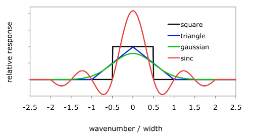
To apply an Instrument Function on SpectralCalc, select the type of function and specify its width W.  We provide a variety of Instrument Function types to choose from:

Here x = σ/W.  (σ  denotes wavenumber).  W is therefore the full width (as opposed to half width).  We constrain W to be no more than 250 cm^‑1, and no more than half of the waveband:

where σ₁ and σ₂ are the lower and upper bounds of the waveband. 

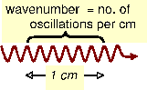
Note that Instrument Functions are always computed and applied in wavenumbers.  A width specified in microns is converted to the equivalent width in wavenumbers at the center of the bandpass.  As a result, an instrument function with its width specified in microns will actually have different effective widths in different spectral bandpasses.

The relative responses of each these functions are shown in Fig. 1. The sinc function is truncated at ±2W, and the Gaussian at ±3W/2.  The triangle's extent is ±W, and the square's is ±W/2.  These functions are sampled at same resolution as the monochromatic spectrum, and normalized to give unit integrated response (i.e. scaled so that the sampled points sum to 1).  The normalization is performed numerically by summing the actual samples of the truncated functions, not by analytically computing the integrals of the underlying continuous functions.  Then the final, smoothed spectrum is computed by a straightforward convolution of the instrument function over the monochromatic spectrum.

Having selected waveband limits σ₁ and σ₂, and an acceptable instrument width W, the smoothed spectrum is resampled with a resolution commensurate with the inputs:

This gives a resolution of 5% of the instrument halfwidth or finer.  It further ensures that the samples evenly divide the user-specified waveband, so that samples occur exactly at σ₁ and σ₂, and at evenly spaced intervals therein.